Principal Component Analysis (PCA)
The PCA tool is used to decrease the dimensionality of the dataset, making it easier to interpret. It accomplishes this via principal components, which are linear combinations of the original dataset. Principal components will begin with a PC 1 value, meaning it is the singular principal component in a one-dimensional space, followed by PC 2 (two-dimensional space), PC 3 (three-dimensional space), and so on. As you lower the number of dimensions, you will naturally lose some data. Explained variance values are included, which signifies how much information is retained at each dimension. Say, for example, you have a ten-dimensional dataset that you want to summarize using two components. To accomplish this, you can use the PC 1 and PC 2 values to do so, with PC 1 holding more significance.
Menu Access: Analysis > PCA
Toolbar Icon: 
Running the Analysis
Go to the
Windowmenu and select one of the data tables. This will bring the selected table window to the front.
Start the PCA tool by clicking on the icon in the toolbar or via the
Analysis>PCAmenu.In the
Configuration: PCAdialog, defineN-components. This variable will control the number of principal components generated by the algroithm. The value will default to 0.999, meaning that the algorithm will stop outputting new components once the 99.9% variance is met. LowerN-componentsvalues will produce a lower number of components.
Check off the boxes for
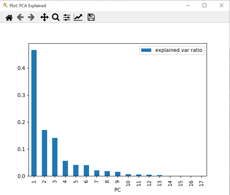
Include original data,Include standardized data, andExplained histogramaccordingly. TheInclude original dataoption will include the original data in the outputted txt file with the principal components, while theInclude standardized dataoption will include the scaled data in that txt file. The ‘Explained histogram` option simply plots the explained variance values on a histogram for visualization.Select the data grouping and data features of interest. Data grouping options are based on the tables category columns, i.e.
Cell,FOV, andTreatmentin this example. Data features correspond to columns with numeric data,FAD a1, etc..In the example, input data is grouped by ‘Cell, FOV, Treatment’, and key data features are selected.
Click
OK.The analysis results are shown in two new data tables, as well as a histogram if the
Explained Histogramcheckbox is checked off. One of the new data tables contains the principal component values for each data point, along with standardized and original data values if selected. The other data table contains the explained variance ratio for each component.
Example Output
Example Results: Data Grouping - Cell, FOV, Treatment
 17 principal components were generated using the default N-components, meaning these 17 PCs reach 99.9% variance.
Histogram with the explained variance values for each principal component: